This page was generated from the Jupyter notebook compare_z_min_cutoff.ipynb.

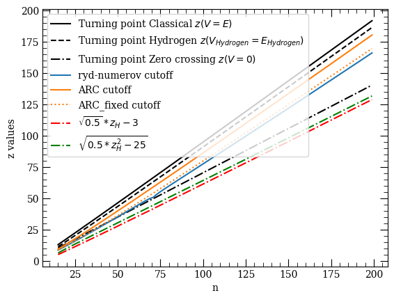
Comparison of the z_min values for circular states to Pairinteraction(v0.9) and ARC

import matplotlib.pyplot as plt
import numpy as np

from ryd_numerov.rydberg import RydbergState

n_list = list(range(15, 200))

qn_list = []
for n in n_list:
    l = {
        "circular": n - 1,
        "intermediate": (n - 1) // 2,
        "s": 0,
        "p": 1,
        "d": 2,
    }["circular"]
    j = l + 0.5
    qn_list.append((n, l, j))

which_turning_point = ["classical", "hydrogen", "zerocrossing"]
z_i_dict = {which: [] for which in which_turning_point}
z_i_dict["ryd-numerov cutoff"] = []
for qn in qn_list:
    print(f"n={qn[0]}", end="\r")
    state = RydbergState("Rb", n=qn[0], l=qn[1], j=qn[2])
    for which in which_turning_point:
        z_i = state.model_potential.calc_z_turning_point(which, dz=1e-3)
        z_i_dict[which].append(z_i)

    state.create_wavefunction()
    z_i_dict["ryd-numerov cutoff"].append(state.wavefunction.grid.z_min)

n=199

import arc
import arc_fixed

atom = arc.Rubidium87()

z_i_dict["ARC cutoff"] = []
z_i_dict["ARC_fixed cutoff"] = []
for use_fixed_arc in [False, True]:
    key = "ARC_fixed cutoff" if use_fixed_arc else "ARC cutoff"
    for qn in qn_list:
        print(f"n={qn[0]}", end="\r")
        r, psi_r = arc_fixed.radialWavefunction(atom, *qn, use_fixed_arc=use_fixed_arc)
        arg_r_min = np.argwhere(psi_r != 0).flatten()[0]
        r_min = r[arg_r_min]
        z_min = np.sqrt(r_min)
        z_i_dict[key].append(z_min)

n=199

fig, ax = plt.subplots()

labels = {
    "classical": "Turning point Classical $z(V=E)$",
    "hydrogen": r"Turning point Hydrogen $z(V_{Hydrogen}=E_{Hydrogen})$",
    "zerocrossing": r"Turning point Zero crossing $z(V=0)$",
}
linestyles = {
    "classical": "-",
    "hydrogen": "--",
    "zerocrossing": "-.",
    "ARC_fixed cutoff": ":",
}
colors = {
    "ryd-numerov cutoff": "C0",
    "ARC cutoff": "C1",
    "ARC_fixed cutoff": "C1",
}

for key, values in z_i_dict.items():
    ax.plot(n_list, values, ls=linestyles.get(key, "-"), color=colors.get(key, "k"), label=labels.get(key, key))

ax.plot(
    n_list,
    np.sqrt(0.5) * np.array(z_i_dict["hydrogen"]) - 3,
    ls="-.",
    color="r",
    label=r"$\sqrt{0.5} * z_H - 3$",
)
ax.plot(
    n_list,
    np.sqrt(0.5 * np.array(z_i_dict["hydrogen"]) ** 2 - 25),
    ls="-.",
    color="green",
    label=r"$\sqrt{0.5 * z_H^2 - 25}$",
)

ax.set_xlabel("n")
ax.set_ylabel("z values")

ax.legend()
plt.show()