This page was generated from the Jupyter notebook mqdt.ipynb.

MQDT Calculations for Ytterbium

The pairinteraction software supports atomic species with two valence electrons such as Yb171 and Yb174, using multi-channel quantum defect theory (MQDT). In the following, we reproduce findings of the publication M. Peper et al., Spectroscopy and modeling of 171Yb Rydberg states for high-fidelity two-qubit gates”, 2024. In this publication, the authors carefully benchmarked their results against experimental data.

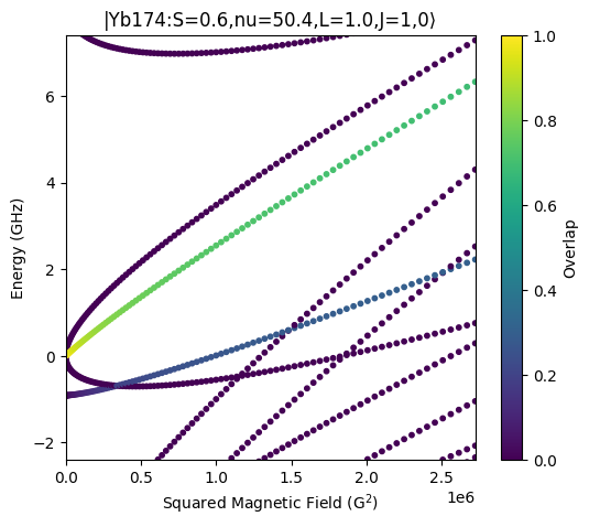
Zeeman Map for Yb174

We calculate the Zeeman map for Yb174 that is shown in Fig. 13 of the publication. The Zeeman map takes into account diamagnetism.

import matplotlib.pyplot as plt
import numpy as np
import pairinteraction.real as pi

if pi.Database.get_global_database() is None:
    pi.Database.initialize_global_database(download_missing=True)

# Get the state of interest
ket = pi.KetAtom("Yb174_mqdt", nu=50, s=1, l=1, j=1, m=0)
energy_in_ghz = ket.get_energy(unit="GHz")

# Construct a basis around the state
basis = pi.BasisAtom("Yb174_mqdt", nu=(ket.nu - 3, ket.nu + 3), j=(0, 2))

# Construct and diagonalize systems for different magnetic fields
list_bfield_in_gauss = np.linspace(0, 1650, 100)
list_system = [
    pi.SystemAtom(basis).set_magnetic_field([0, 0, b], unit="G").set_diamagnetism_enabled(True)
    for b in list_bfield_in_gauss
]
pi.diagonalize(list_system, diagonalizer="lapacke_evd", float_type="float32")

# Get eigenenergies and overlaps
list_eigenenergies = np.array([system.get_eigenenergies(unit="GHz") for system in list_system])
list_overlap = np.array([system.get_eigenbasis().get_overlaps(ket) for system in list_system])

# Plot the Zeeman map
fig = plt.figure(figsize=(6, 5))
ax = fig.add_subplot(111)
ax.set_title(ket.get_label("ket"))
scat = ax.scatter(
    np.repeat(list_bfield_in_gauss, list_eigenenergies.shape[1]) ** 2,
    list_eigenenergies - energy_in_ghz,
    c=list_overlap,
    s=10,
    vmin=0,
    vmax=1,
)
fig.colorbar(scat, label="Overlap")
ax.set_xlim(0, list_bfield_in_gauss[-1] ** 2)
ax.set_ylim(-2.4, 7.4)
ax.set_xlabel(r"Squared Magnetic Field (G$^2$)")
ax.set_ylabel("Energy (GHz)")
plt.show()

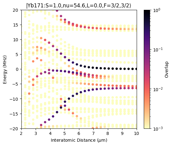
Pair Potentials for Yb171

We calculate the pair potentials for Yb171 that are displayed in Fig. 7a of the publication. The pair potentials are calculated for a magnetic field pointing along the z-axis and the interatomic axis pointing along the x-axis. Because this arrangement breaks rotational symmetry, the total magnetic quantum number is not conserved and two-atom Hilbert space is rather large. To keep the execution time down, we only calculate the pair potentials for a few interatomic distances.

import matplotlib.pyplot as plt
import numpy as np
import pairinteraction.real as pi

if pi.Database.get_global_database() is None:
    pi.Database.initialize_global_database(download_missing=True)

# Get the state of interest
ket = pi.KetAtom("Yb171_mqdt", nu=54.56, l=0, f=3 / 2, m=3 / 2)

# Construct a basis around the state
basis = pi.BasisAtom("Yb171_mqdt", nu=(ket.nu - 2, ket.nu + 2), f=(0.5, 2.5))

# Construct and diagonalize a system for a single atom
system = (
    pi.SystemAtom(basis)
    .set_magnetic_field([0, 0, 5.03], unit="G")
    .set_diamagnetism_enabled(True)
    .diagonalize(diagonalizer="lapacke_evr", float_type="float32")
)
pair_energy_shifted = 2 * system.get_corresponding_energy(ket, unit="MHz")

# Construct a basis for a pair of atoms
basis_pair = pi.BasisPair(
    [system, system],
    energy=(pair_energy_shifted - 3.5e3, pair_energy_shifted + 3.5e3),
    energy_unit="MHz",
)
print(f"Pair basis size: {basis_pair.number_of_states}", flush=True)

# Construct and diagonalize systems for different interatomic distances
list_distances = np.linspace(2, 10, 30)
list_system = [
    pi.SystemPair(basis_pair).set_distance_vector([d, 0, 0], unit="um") for d in list_distances
]
pi.diagonalize(
    list_system,
    diagonalizer="lapacke_evr",
    float_type="float32",
    energy_range=(pair_energy_shifted - 20, pair_energy_shifted + 20),
    energy_unit="MHz",
    rtol=1e-6,
)

# Get eigenenergies and overlaps
list_eigenenergies = [system.get_eigenenergies(unit="MHz") for system in list_system]
list_overlap = [system.get_eigenbasis().get_overlaps([ket, ket]) for system in list_system]
list_distances = [d * np.ones_like(e) for d, e in zip(list_distances, list_eigenenergies)]

# Plot the pair potential
list_eigenenergies = np.hstack(list_eigenenergies)
list_overlap = np.hstack(list_overlap)
list_distances = np.hstack(list_distances)
sorter = np.argsort(list_overlap)

fig = plt.figure(figsize=(6, 5))
ax = fig.add_subplot(111)
ax.set_title(ket.get_label("ket"))
scat = ax.scatter(
    list_distances[sorter],
    list_eigenenergies[sorter] - pair_energy_shifted,
    c=list_overlap[sorter],
    s=20,
    vmin=1e-3,
    vmax=1,
    norm="log",
    cmap="magma_r",
)
fig.colorbar(scat, label="Overlap")
ax.set_xlim(2, 10)
ax.set_ylim(-20, 20)
ax.set_xlabel(r"Interatomic Distance ($\mu$m)")
ax.set_ylabel("Energy (MHz)")
plt.show()

Pair basis size: 3392