This page was generated from the Jupyter notebook perturbative_h_eff.ipynb.

Effective Hamiltonian

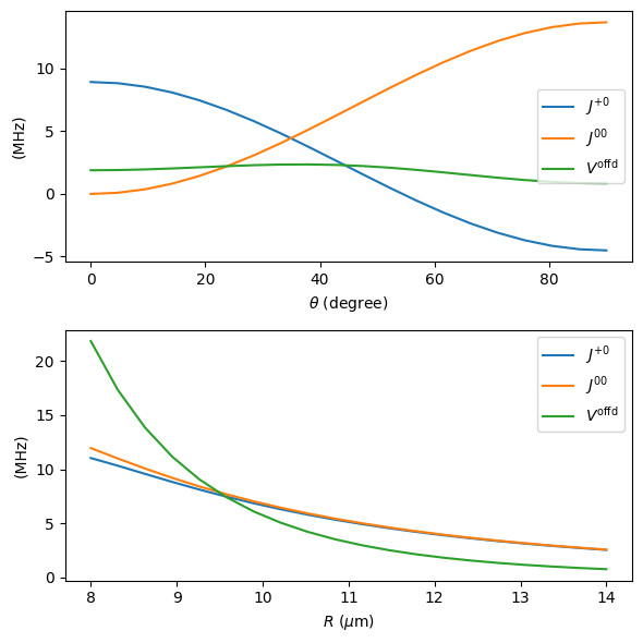
This notebook demonstrates how to calculate an effective Hamiltonian with the pairinteraction.perturbative module. We use https://arxiv.org/pdf/2410.21424 as a reference and try to reproduce figure 2c) and d) from the paper. Note that the paper used a Schrieffer-Wolff transformation to calculate the effective Hamiltonian, while here we use perturbation theory up to third order.

import logging

import matplotlib.pyplot as plt
import numpy as np
import pairinteraction.real as pi
from pairinteraction import perturbative

logging.basicConfig(level=logging.ERROR)

if pi.Database.get_global_database() is None:
    pi.Database.initialize_global_database(download_missing=True)

kets = {
    "+": pi.KetAtom("Rb", n=81, l=0, j=0.5, m=0.5),
    "0": pi.KetAtom("Rb", n=80, l=1, j=1.5, m=1.5),
    "-": pi.KetAtom("Rb", n=80, l=0, j=0.5, m=0.5),
}
pair_energy = kets["0"].get_energy("GHz") * 2

basis = pi.BasisAtom(
    species="Rb",
    n=(78, 83),
    l=(0, 2),
    j=(0.5, 4.5),
)

system = pi.SystemAtom(basis=basis)
system.set_diamagnetism_enabled(True)
system.set_magnetic_field([0, 0, 60.7], "gauss")
system.diagonalize()

delta_energy = 5  # GHZ
basis_pair = pi.BasisPair(
    [system, system],
    energy=(pair_energy - delta_energy, pair_energy + delta_energy),
    energy_unit="GHz",
)
system_pair = pi.SystemPair(basis_pair)
system_pair.set_interaction_order(3)

SystemPairReal(BasisPairReal(|Rb:78,S_1/2,-1/2; Rb:83,S_1/2,-1/2⟩ ... |Rb:83,P_3/2,3/2; Rb:78,S_1/2,1/2⟩), is_diagonal=True)

theta_list = np.linspace(0, 90, 20)  # degree
R_list = np.linspace(8, 14, 20)  # mum

theta_default = 35.1  # rad
R_default = 11.6  # mum

order = 3

kets_list = [(kets["+"], kets["-"]), (kets["0"], kets["0"]), (kets["-"], kets["+"])]
H_eff = {"theta": [], "R": []}

for theta in theta_list:
    system_pair.set_distance_vector(
        R_default * np.array([np.sin(theta * np.pi / 180), 0, np.cos(theta * np.pi / 180)]),
        "micrometer",
    )
    h_eff, _ = perturbative.get_effective_hamiltonian_from_system(
        kets_list, system_pair, order, unit="MHz"
    )
    H_eff["theta"].append(h_eff)

for R in R_list:
    system_pair.set_distance_vector(
        R
        * np.array(
            [np.sin(theta_default * np.pi / 180), 0, np.cos(theta_default * np.pi / 180)]
        ),
        "micrometer",
    )
    h_eff, _ = perturbative.get_effective_hamiltonian_from_system(
        kets_list, system_pair, order, unit="MHz"
    )
    H_eff["R"].append(h_eff)

pair_energy = kets["+"].get_energy("GHz") + kets["0"].get_energy("GHz")
basis_pair = pi.BasisPair(
    [system, system],
    energy=(pair_energy - delta_energy, pair_energy + delta_energy),
    energy_unit="GHz",
)
system_pair = pi.SystemPair(basis_pair)
system_pair.set_interaction_order(3)

kets_list = [(kets["+"], kets["0"]), (kets["0"], kets["+"])]
H_eff_p0 = {"theta": [], "R": []}

for theta in theta_list:
    system_pair.set_distance_vector(
        R_default * np.array([np.sin(theta * np.pi / 180), 0, np.cos(theta * np.pi / 180)]),
        "micrometer",
    )
    h_eff, _ = perturbative.get_effective_hamiltonian_from_system(
        kets_list, system_pair, order, unit="MHz"
    )
    H_eff_p0["theta"].append(h_eff)

for R in R_list:
    system_pair.set_distance_vector(
        R
        * np.array(
            [np.sin(theta_default * np.pi / 180), 0, np.cos(theta_default * np.pi / 180)]
        ),
        "micrometer",
    )
    h_eff, _ = perturbative.get_effective_hamiltonian_from_system(
        kets_list, system_pair, order, unit="MHz"
    )
    H_eff_p0["R"].append(h_eff)

H_eff = {key: np.array(value) for key, value in H_eff.items()}
H_eff_p0 = {key: np.array(value) for key, value in H_eff_p0.items()}

fig, axs = plt.subplots(2, 1, figsize=(6, 6))

axs[0].plot(theta_list, H_eff_p0["theta"][:, 0, 1], "C0-", label=r"$J^{+0}$")
axs[0].plot(theta_list, H_eff["theta"][:, 0, 1], "C1-", label=r"$J^{00}$")
axs[0].plot(theta_list, H_eff["theta"][:, 0, 2], "C2-", label=r"$V^\text{offd}$")
axs[0].set_xlabel(r"$\theta$ (degree)")

axs[1].plot(R_list, H_eff_p0["R"][:, 0, 1], "C0-", label=r"$J^{+0}$")
axs[1].plot(R_list, H_eff["R"][:, 0, 1], "C1-", label=r"$J^{00}$")
axs[1].plot(R_list, H_eff["R"][:, 0, 2], "C2-", label=r"$V^\text{offd}$")
axs[1].set_xlabel(r"$R$ ($\mu$m)")

for ax in axs:
    ax.legend()
    ax.set_ylabel(r"(MHz)")

fig.tight_layout()
plt.show()