This page was generated from the Jupyter notebook lifetimes.ipynb. Open in Google Colab.

Lifetimes

We calculate the lifetime of Rydberg states and analyze which transitions contribute to it. The calculations can be performed with a few lines of code; most of the code within this notebook is only needed for plotting.

We import the libraries that we will use within the notebook and initialize PairInteraction’s database.

%pip install -q matplotlib numpy scipy pairinteraction

from typing import Any

import matplotlib.pyplot as plt
import numpy as np
import pairinteraction as pi
from scipy.optimize import curve_fit

if pi.Database.get_global_database() is None:
    pi.Database.initialize_global_database(download_missing=True)

As a quick example, we show how to calculate the lifetime of the Rubidium \(|60S,m=1/2\rangle\) state via ket.get_lifetime. At zero temperature, the lifetime is determined by the spontaneous decay. If the temperature is non-zero, black body radiation can drive transitions to neighboring Rydberg states, reducing the lifetime.

ket = pi.KetAtom("Rb", n=60, l=0, j=0.5, m=0.5)

temperature = 300  # Kelvin
lifetime_0 = ket.get_lifetime()
lifetime = ket.get_lifetime(temperature, temperature_unit="K")

print(f"Lifetime at T=0: {lifetime_0.to('mus'):.2f}")
print(f"Lifetime at T={temperature}K: {lifetime.to('mus'):.2f}")

The single-channel quantum defect theory can be inaccurate for effective principal quantum numbers < 25. This can lead to inaccurate matrix elements.
The single-channel quantum defect theory can be inaccurate for effective principal quantum numbers < 25. This can lead to inaccurate matrix elements.
The single-channel quantum defect theory can be inaccurate for effective principal quantum numbers < 25. This can lead to inaccurate matrix elements.

Lifetime at T=0: 239.07 microsecond
Lifetime at T=300K: 104.73 microsecond

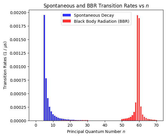
Transition rates contributing to the Rydberg lifetime

To analyze which transitions contribute to the lifetime, we can obtain the transition rates from spontaneous decay (ket.get_spontaneous_transition_rates) and black body radiation (ket.get_black_body_transition_rates).

# Calculate the transition rates
kets_sp, transition_rates_sp = ket.get_spontaneous_transition_rates(unit="1/mus")
print(f"Number of possible spontaneous decay transitions: {len(transition_rates_sp)}")

kets_bbr, transition_rates_bbr = ket.get_black_body_transition_rates(
    temperature, "kelvin", unit="1/mus"
)
print(f"Number of considered BBR transitions: {len(transition_rates_bbr)}")

# Plot the transition rates
fig, ax = plt.subplots(figsize=(6, 5))

n_list = np.arange(0, np.max([s.n for s in kets_bbr]) + 1)
rates_summed = {}
for key, kets, rates in [
    ("BBR", kets_bbr, transition_rates_bbr),
    ("SP", kets_sp, transition_rates_sp),
]:
    rates_summed[key] = np.zeros(len(n_list))
    for i, s in enumerate(kets):
        rates_summed[key][s.n] += rates[i]

ax.bar(n_list, rates_summed["SP"], label="Spontaneous Decay", color="blue", alpha=0.8)
ax.bar(n_list, rates_summed["BBR"], label="Black Body Radiation (BBR)", color="red", alpha=0.8)
ax.legend()

ax.set_xlabel("Principal Quantum Number $n$")
ax.set_ylabel(r"Transition Rates (1 / $\mu$s)")
ax.set_title("Spontaneous and BBR Transition Rates vs $n$")

plt.show()

The single-channel quantum defect theory can be inaccurate for effective principal quantum numbers < 25. This can lead to inaccurate matrix elements.
The single-channel quantum defect theory can be inaccurate for effective principal quantum numbers < 25. This can lead to inaccurate matrix elements.

Number of possible spontaneous decay transitions: 180
Number of considered BBR transitions: 235

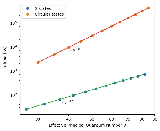
Lifetime scaling with the principal quantum number

As a more sophisticated example, we study how the lifetime scales with the effective principal quantum number \(\nu\). Our numerics reproduce the \(\nu^3\) scaling which one expects for states with a small angular quantum number \(l\). For circular states, the lifetime scales as \(\nu^5\).

n_list = list(range(30, 90, 5))


def fit_function(x: np.ndarray, a: float, b: float) -> np.typing.NDArray[Any]:
    return a * x + b


# Calculate lifetimes for S states
kets_s = [pi.KetAtom("Rb", n=n, l=0, j=0.5, m=0.5) for n in n_list]
nu_s = [ket.nu for ket in kets_s]
lifetimes_s = [ket.get_lifetime(unit="mus") for ket in kets_s]
popt_s, _ = curve_fit(fit_function, np.log(nu_s), np.log(lifetimes_s))

# Calculate lifetimes for circular states
kets_circular = [pi.KetAtom("Rb", n=n, l=n - 1, j=n - 0.5, m=n - 0.5) for n in n_list]
nu_circular = [ket.nu for ket in kets_circular]
lifetimes_circular = [ket.get_lifetime(unit="mus") for ket in kets_circular]
popt_circular, _ = curve_fit(fit_function, np.log(nu_circular), np.log(lifetimes_circular))

# Plot the scaling of the lifetimes
fig, ax = plt.subplots(figsize=(6, 5))

ax.plot(nu_s, lifetimes_s, "o", label="S states")
ax.plot(nu_circular, lifetimes_circular, "o", label="Circular states")

fit_s = np.exp(fit_function(np.log(nu_s), *popt_s))
fit_circular = np.exp(fit_function(np.log(nu_circular), *popt_circular))
ax.plot(nu_s, fit_s)
ax.plot(nu_circular, fit_circular)

ax.text(nu_s[2], fit_s[2], rf"$\propto \nu^{{{popt_s[0]:.2f}}}$", verticalalignment="top")
ax.text(
    nu_circular[2],
    fit_circular[2],
    rf"$\propto \nu^{{{popt_circular[0]:.2f}}}$",
    verticalalignment="top",
)

ax.legend()
ax.set_yscale("log")
ax.set_xscale("log")
ax.set_xlabel(r"Effective Principal Quantum Number $\nu$")
ax.set_ylabel(r"Lifetime ($\mu$s)")

ax.set_xticks([30, 40, 50, 60, 70, 80, 90])
ax.get_xaxis().set_major_formatter(plt.ScalarFormatter())

plt.show()