This page was generated from the Jupyter notebook compare_model_potentials.ipynb.

Compare different effective model potentials

import matplotlib.pyplot as plt

import rydstate

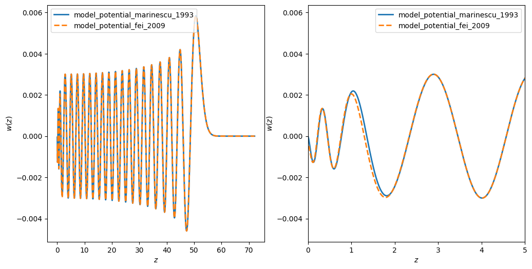
Check Rubidium with large n

For Rubidium and large quantum numbers n we expect the effective model potentials to be very similar.

species, n, l, j = "Rb", 40, 0, 0.5
state = rydstate.RydbergStateSQDTAlkali(species, n, l=l, j=j)

states: dict[str, rydstate.RydbergStateSQDTAlkali] = {}
states["marinescu_1994"] = rydstate.RydbergStateSQDTAlkali(species, n, l=l, j=j, potential="marinescu_1994")
states["fei_2009"] = rydstate.RydbergStateSQDTAlkali(species, n, l=l, j=j, potential="fei_2009")

for label, state in states.items():
    print(f"Integrating wavefunction for {label}")
    state.radial.integrate_wavefunction()

Integrating wavefunction for marinescu_1994
Integrating wavefunction for fei_2009

fig, axs = plt.subplots(1, 2, figsize=(12, 6))

for ax in axs:
    linestyles = ["-", "--", "-.", ":"]
    for label, state in states.items():
        ax.plot(state.radial.z_list, state.radial.w_list, label=label, lw=2, ls=linestyles.pop(0))

    ax.legend()
    ax.set_xlabel("$z$")
    ax.set_ylabel("$w(z)$")

axs[1].set_xlim(0, 5)

plt.show()

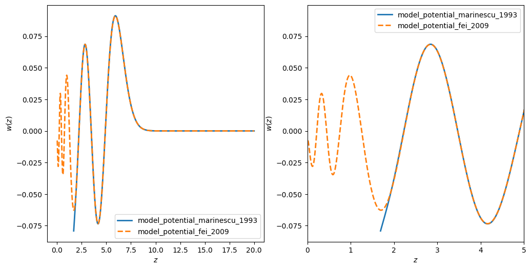
Big differences for Strontium with small n

state = rydstate.RydbergStateSQDT("Sr88", n=8, l_r=0, j_tot=0, s_tot=0)

states = {}
states["marinescu_1994"] = rydstate.RydbergStateSQDT(
    state.species, n=state.n, angular_ket=state.angular, potential="marinescu_1994"
)
states["fei_2009"] = rydstate.RydbergStateSQDT(
    state.species, n=state.n, angular_ket=state.angular, potential="fei_2009"
)

for label, state in states.items():
    print(f"Integrating wavefunction for {label}")
    state.radial.integrate_wavefunction()

The wavefunction for the radial_ket RadialKet(nu=4.742213450510572, potential=PotentialMarinescu1994Strontium88(l_r=0)) has some issues:
      The wavefunction is not close to zero at the inner boundary (inner_weight_scaled_to_whole_grid=5.99e-01)
      The wavefunction has 3 nodes, but should have 7 nodes.
      The integration for l=0 did stop at 1.69 (should be close to zero).

Integrating wavefunction for marinescu_1994
Integrating wavefunction for fei_2009

fig, axs = plt.subplots(1, 2, figsize=(12, 6))

for ax in axs:
    linestyles = ["-", "--", "-.", ":"]
    for label, state in states.items():
        ax.plot(state.radial.z_list, state.radial.w_list, label=label, lw=2, ls=linestyles.pop(0))

    ax.legend()
    ax.set_xlabel("$z$")
    ax.set_ylabel("$w(z)$")

axs[1].set_xlim(0, 5)

plt.show()