This page was generated from the Jupyter notebook compare_nist_matrix_elements.ipynb.

Compare Rb \(5s \rightarrow np_j\) matrix elements with NIST

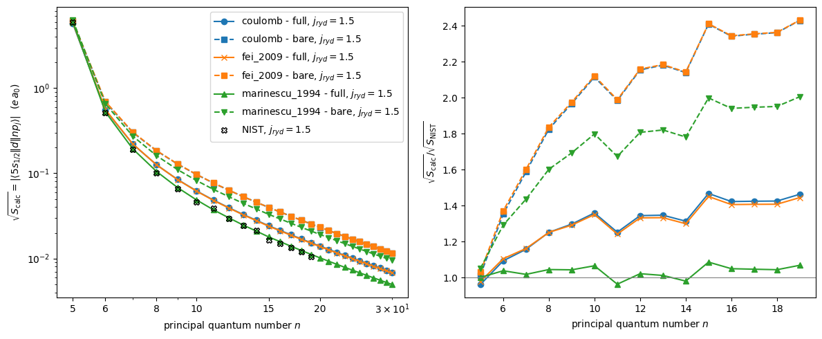
This notebook compares the reduced electric-dipole matrix elements \(\langle 5s_{1/2} \Vert d \Vert np_j \rangle\) of rubidium (\(n = 5, \dots, 20\) and \(j = 1/2, 3/2\)) computed by rydstate with the experimental values of the NIST Atomic Spectra Database (ASD), for

• the bare rydberg dipole operator \(d(r) = r\), and

• the full (core-polarization dressed) dipole operator \(d(r) = r - \frac{\alpha_c}{r^2}\left(1 - e^{-(r/r_c)^3}\right)\).

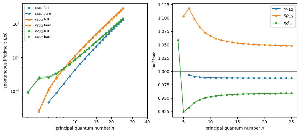
The later sections then look at how the full operator affects the remaining decay channels of the \(np\) states and, finally, the \(ns_{1/2}\), \(np_{3/2}\) and \(nd_{5/2}\) lifetimes. For those no NIST line strengths are used, so there only the bare and full values are compared to each other.

The valence electron polarizes the ionic core; the induced core dipole partially shields the dipole operator. This correction goes back to Hameed et al J. Phys. B: Atom. Mol. Phys. 1 822, 1962 and Weisheit Phys. Rev. A 5, 1621, 1972, and is also described in Marinescu et al Phys. Rev. A 49, 982, 1994, where the model potential comes from. The cutoff \(r_c\) is fitted to the NIST line strengths.

# %matplotlib widget

import logging

import matplotlib.pyplot as plt
import numpy as np

import rydstate

logging.getLogger("rydstate").setLevel(logging.ERROR)

NIST reference values

The NIST ASD line strength of an E1 transition is \(S = |\langle J \Vert d \Vert J' \rangle|^2\) in atomic units \((e\,a_0)^2\), so it is directly comparable to the square of rydstate’s reduced matrix elements.

# {(n, j): S in (e a0)^2} from https://physics.nist.gov/PhysRefData/ASD/lines_form.html (retrieved 2026-07-24)
nist_s = {
    (5, 0.5): 1.79e1,
    (6, 0.5): 1.11e-1,
    (7, 0.5): 1.32e-2,
    (8, 0.5): 3.31e-3,
    (9, 0.5): 1.28e-3,
    (10, 0.5): 6.24e-4,
    (11, 0.5): 3.79e-4,
    (12, 0.5): 2.02e-4,
    (13, 0.5): 1.28e-4,
    (14, 0.5): 1.04e-4,
    (15, 0.5): 6.85e-5,
    (16, 0.5): 4.82e-5,
    (17, 0.5): 3.75e-5,
    (18, 0.5): 2.83e-5,
    (19, 0.5): 2.34e-5,
    (20, 0.5): 1.50e-5,
    (5, 1.5): 3.58e1,
    (6, 1.5): 2.59e-1,
    (7, 1.5): 3.62e-2,
    (8, 1.5): 1.01e-2,
    (9, 1.5): 4.25e-3,
    (10, 1.5): 2.10e-3,
    (11, 1.5): 1.50e-3,
    (12, 1.5): 8.62e-4,
    (13, 1.5): 5.95e-4,
    (14, 1.5): 4.57e-4,
    (15, 1.5): 2.72e-4,
    (16, 1.5): 2.25e-4,
    (17, 1.5): 1.77e-4,
    (18, 1.5): 1.42e-4,
    (19, 1.5): 1.10e-4,
}

Bare vs. full operator

The full operator (including the core-polarization correction) is used automatically if “electric_dipole” is specified. To compute the bare values for comparison, one can restrict the matrix element to the contribution of the Rydberg electron via part="rydberg", which leaves out the “closed_shell_core” contribution.

n_max = 30
matrix_elements: dict[str, dict[tuple[int, float], float]] = {}

for potential in ["coulomb", "fei_2009", "marinescu_1994"]:
    basis_ns = rydstate.BasisSQDT("Rb", n=(0, n_max), l_r=(0, 0), potential_class=potential)
    ground_state = basis_ns.sort_states("nu").states[0]
    basis_np = rydstate.BasisSQDT("Rb", n=(0, n_max), l_r=(1, 1), potential_class=potential)

    matrix_elements[potential + " - full"] = {
        (state.n, state.calc_exp_qn("j_r")): state.calc_reduced_matrix_element(
            ground_state, "electric_dipole", unit="e a0"
        )
        for state in basis_np.states
    }

    matrix_elements[potential + " - bare"] = {
        (state.n, state.calc_exp_qn("j_r")): state.calc_reduced_matrix_element(
            ground_state, "electric_dipole", part="rydberg", unit="e a0"
        )
        for state in basis_np.states
    }

Comparison plot

Left: the matrix elements themselves. Right: the ratio of the calculated matrix elements to the NIST values. The color encodes the total angular momentum (\(j = 1/2\) blue, \(j = 3/2\) orange), and the black-edged crosses the NIST values. The bare operator overestimates the matrix elements; the full operator agrees with the NIST values.

fig, (ax_me, ax_ratio) = plt.subplots(1, 2, figsize=(12, 5))

colors = ["C0", "C0", "C1", "C1", "C2", "C2", "C3", "C3"]
linestyles = ["-", "--", "-", "--", "-", "--", "-", "--"]
markers = ["o", "s", "x", "s", "^", "v", "o", "s", "^", "v"]

j_r = 3 / 2
j_r_label = rf"$j_{{ryd}}={j_r}$"
n_nist = sorted(n for (n, _j_r) in nist_s if _j_r == j_r)

for label, me in matrix_elements.items():
    n_list = [n for (n, _j_r) in me if _j_r == j_r]
    style = {"color": colors.pop(0), "linestyle": linestyles.pop(0), "marker": markers.pop(0), "markersize": 6}
    ax_me.plot(n_list, [abs(me[(n, j_r)]) for n in n_list], **style, label=f"{label}, {j_r_label}")
    ax_ratio.plot(n_nist, np.abs([me[(n, j_r)] / np.sqrt(nist_s[(n, j_r)]) for n in n_nist]), **style)

ax_me.plot(
    n_nist,
    [np.sqrt(nist_s[(n, j_r)]) for n in n_nist],
    color="k",
    linestyle="none",
    marker="X",
    markeredgecolor="black",
    fillstyle="none",
    label=f"NIST, {j_r_label}",
)

ax_me.set_xscale("log")
ax_me.set_yscale("log")
ax_me.set_xticks([5, 6, 8, 10, 15, 20], labels=["5", "6", "8", "10", "15", "20"])
ax_me.set_xlabel("principal quantum number $n$")
ax_me.set_ylabel(r"$\sqrt{S_\mathrm{calc}} = |\langle 5s_{1/2} \Vert d \Vert np_j \rangle|$  ($e\,a_0$)")
ax_me.legend()

ax_ratio.axhline(1, color="gray", lw=0.8)
ax_ratio.set_xlabel("principal quantum number $n$")
ax_ratio.set_ylabel(r"$\sqrt{S_\mathrm{calc}} / \sqrt{S_\mathrm{NIST}}$")

fig.tight_layout()
plt.show()

Why lifetimes barely change: the \(np \rightarrow\) low-\(n\) \(d\) and \(s\) channels

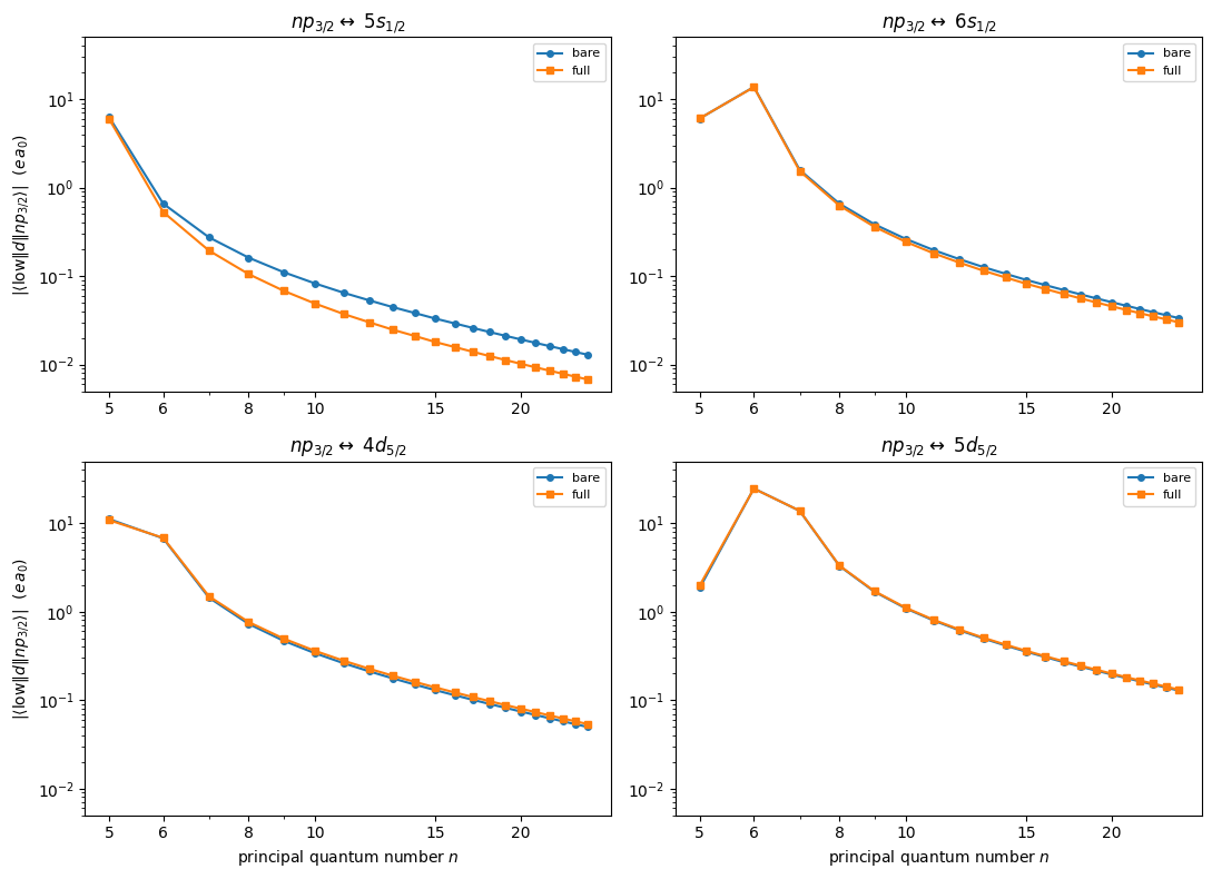
The line strengths \(S\) to the ground state change by up to a factor \(\sim 8\), yet the lifetimes of Rydberg \(np\) states change only by a few percent. The reason becomes clear by looking at how the full operator affects the other decay channels of an \(np_{3/2}\) state: the dominant spontaneous channels go to the low-lying \(d\) states, whose radial integrals have no strong cancellation — so the shielding correction moves them only mildly. Below we first plot the bare and full matrix elements for the four most important channel families, and then the ratio of the full to the bare line strength for all of them in a single plot.

low_n = 5
lower_states = {
    rf"${low_n}s_{{1/2}}$": rydstate.RydbergStateSQDTAlkali("Rb", low_n, l=0, j=0.5),
    rf"${low_n + 1}s_{{1/2}}$": rydstate.RydbergStateSQDTAlkali("Rb", low_n + 1, l=0, j=0.5),
    rf"${low_n - 1}d_{{5/2}}$": rydstate.RydbergStateSQDTAlkali("Rb", low_n - 1, l=2, j=2.5),
    rf"${low_n}d_{{5/2}}$": rydstate.RydbergStateSQDTAlkali("Rb", low_n, l=2, j=2.5),
}
basis_np = rydstate.BasisSQDT("Rb", n=(0, 25), l_r=(1, 1), f_tot=(1.5, 1.5))

fig, axes = plt.subplots(2, 2, figsize=(11, 8))

for ax, label in zip(axes.flat, lower_states, strict=True):
    n_list = basis_np.calc_exp_qn("n")
    me_bare_low = basis_np.calc_reduced_matrix_element(
        lower_states[label], "electric_dipole", part="rydberg", unit="e a0"
    )
    ax.plot(n_list, np.abs(me_bare_low), "C0o-", markersize=4, label="bare")
    me_full_low = basis_np.calc_reduced_matrix_element(lower_states[label], "electric_dipole", unit="e a0")
    ax.plot(n_list, np.abs(me_full_low), "C1s-", markersize=4, label="full")

    ax.set_xscale("log")
    ax.set_yscale("log")
    ax.set_ylim(5e-3, 5e1)
    ax.set_xticks([5, 6, 8, 10, 15, 20], labels=["5", "6", "8", "10", "15", "20"])
    ax.set_title(rf"$np_{{3/2}} \leftrightarrow$ {label}")
    ax.legend(fontsize=8)

for ax in axes[-1]:
    ax.set_xlabel("principal quantum number $n$")
for ax in axes[:, 0]:
    ax.set_ylabel(r"$|\langle \mathrm{low} \Vert d \Vert np_{3/2} \rangle|$  ($e\,a_0$)")

fig.tight_layout()
plt.show()

fig, ax = plt.subplots(figsize=(7, 4.5))

for i, label in enumerate(lower_states):
    n_list = basis_np.calc_exp_qn("n")
    me_bare_low = basis_np.calc_reduced_matrix_element(
        lower_states[label], "electric_dipole", part="rydberg", unit="e a0"
    )
    me_full_low = basis_np.calc_reduced_matrix_element(lower_states[label], "electric_dipole", unit="e a0")
    ax.plot(
        n_list,
        np.abs(me_full_low / me_bare_low),
        f"C{i}o-",
        markersize=4,
        label=rf"$np_{{3/2}} \leftrightarrow$ {label}",
    )

ax.axhline(1, color="gray", lw=0.8)
ax.set_xlabel("principal quantum number $n$")
ax.set_ylabel(r"$\sqrt{S_\mathrm{full}} / \sqrt{S_\mathrm{bare}}$")
ax.legend()

plt.show()

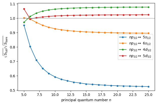
The \(np \rightarrow 5s\) line strengths are suppressed down to $:nbsphinx-math:sim`$0.3 (and the :math:`np_{1/2} ones even further, cf. the plot above), but this channel carries only a modest share of the total decay rate. The dominant \(np \rightarrow 4d, 5d\) channels move by at most $:nbsphinx-math:sim`$15%, partly in the *opposite* direction (the full operator enhances these partially-cancelling integrals), and transitions between neighboring Rydberg states (large :math:`r, no cancellation) are untouched. The net effect on the \(np_{3/2}\) lifetimes is a few percent — worked out in detail below.

Lifetimes vs. principal quantum number

We compute the spontaneous (\(T = 0\)) lifetimes of the \(ns_{1/2}\), \(np_{3/2}\) and \(nd_{5/2}\) series with the default (full) operator and with the bare operator.

series = {
    "$ns_{1/2}$": rydstate.BasisSQDT("Rb", n=(6, 25), l_r=(0, 0), f_tot=(0.5, 0.5), m=(0.5, 0.5)),
    "$np_{3/2}$": rydstate.BasisSQDT("Rb", n=(0, 25), l_r=(1, 1), f_tot=(1.5, 1.5), m=(0.5, 0.5)),
    "$nd_{5/2}$": rydstate.BasisSQDT("Rb", n=(0, 25), l_r=(2, 2), f_tot=(2.5, 2.5), m=(0.5, 0.5)),
}

lifetimes_full = {label: [state.get_lifetime(unit="us") for state in basis.states] for label, basis in series.items()}

element_properties = rydstate.species.rubidium.ElementPropertiesRubidium
alpha_closed_shell_core = element_properties.alpha_closed_shell_core
element_properties.alpha_closed_shell_core = 0  # ignore core polarizability for bare lifetime
rydstate.radial.RadialKet.clear_cached_instances()

lifetimes_bare = {label: [state.get_lifetime(unit="us") for state in basis.states] for label, basis in series.items()}

rydstate.radial.RadialKet.clear_cached_instances()
element_properties.alpha_closed_shell_core = alpha_closed_shell_core  # restore core polarizability

fig, (ax_tau, ax_ratio) = plt.subplots(1, 2, figsize=(12, 5))

for i, (label, basis) in enumerate(series.items()):
    n_list = basis.calc_exp_qn("n")
    ax_tau.plot(n_list, lifetimes_full[label], f"C{i}o-", markersize=4, label=f"{label} full")
    ax_tau.plot(n_list, lifetimes_bare[label], f"C{i}o--", fillstyle="none", markersize=4, label=f"{label} bare")
    ratio = np.array(lifetimes_full[label]) / np.array(lifetimes_bare[label])
    ax_ratio.plot(n_list, ratio, f"C{i}o-", markersize=4, label=label)

ax_tau.set_xscale("log")
ax_tau.set_yscale("log")
ax_tau.set_xticks([10, 15, 20, 30, 40], labels=["10", "15", "20", "30", "40"])
ax_tau.set_xlabel("principal quantum number $n$")
ax_tau.set_ylabel(r"spontaneous lifetime $\tau$ ($\mu$s)")
ax_tau.legend(fontsize=8)

ax_ratio.axhline(1, color="gray", lw=0.8)
ax_ratio.set_xlabel("principal quantum number $n$")
ax_ratio.set_ylabel(r"$\tau_\mathrm{full} / \tau_\mathrm{bare}$")
ax_ratio.legend()

plt.show()