This page was generated from the Jupyter notebook effective_hamiltonian.ipynb. Open in Google Colab.

Effective Hamiltonian

The PairInteraction Python API comes with high-level functionality to calculate effective Hamiltonians (up to 3rd order perturbation theory) without having to write much code. All functionality for this is provided by the pi.EffectiveSystemPair class.

If you are only interested in calculating C3 or C6 coefficients, you can also use the specialized pi.C3 and pi.C6 classes directly, see the tutorial C3 and C6 coefficients.

The pi.EffectiveSystemPair class can be used as follows:

• The constructor of this class takes a list of pair states of interest, wich can be specified by passing a tuple of two pi.KetAtom objects for each pair state.

• The set_distance method sets the distance between the two atoms

• If the effective Hamiltonian should be calculated in the presence of e.g. a magnetic field, the set_magnetic_field method can be used. In general, this class supports similar setters as the pi.SystemAtom and pi.SystemPair classes.

• The get_effective_hamiltonian method returns the effective Hamiltonian.

• This class determines automatically which states should be taken into account to obtain an accurate effective Hamiltonian. To provide guidance how many states in the pair basis should be considered, you can use the method set_minimum_number_of_ket_pairs and set_maximum_number_of_ket_pairs.

%pip install -q matplotlib numpy pairinteraction

import matplotlib.pyplot as plt
import numpy as np
import pairinteraction as pi

if pi.Database.get_global_database() is None:
    pi.Database.initialize_global_database(download_missing=True)

Quickly get an effective Hamiltonian for a pair of Rydberg atoms

In the following, we have a minimal example for calculating an effective Hamiltonian.

ket1 = pi.KetAtom("Rb", n=61, l=0, j=0.5, m=0.5)
ket2 = pi.KetAtom("Rb", n=62, l=1, j=1.5, m=0.5)

eff_h_obj = pi.EffectiveSystemPair([(ket1, ket2), (ket2, ket1)])
eff_h_obj.set_perturbation_order(2)
eff_h_obj.set_magnetic_field([0, 0, 20], "gauss")
eff_h_obj.set_distance(10, unit="micrometer")
eff_h = eff_h_obj.get_effective_hamiltonian(unit="GHz")
eff_h -= np.eye(2) * eff_h_obj.get_pair_energies("GHz")[0]  # shift energy

print("Effective Hamiltonian in GHz:")
print(eff_h)

Effective Hamiltonian in GHz:
[[-8.32562800e-05 -1.04118184e-04]
 [-1.04118184e-04 -8.32562800e-05]]

Get an effective Hamiltonian for a spin-1 like (three level) system

As a more advanced example, we consider a spin-1 like system as described in PRX Quantum 6, 020332 (2025) and try to reproduce figure 2c) and d) from that paper. Note that the paper used a Schrieffer-Wolff transformation to calculate the effective Hamiltonian, while here we use perturbation theory up to third order.

Let us start by defining all single-atom states of interest, as well as the fields and distances between the atoms used in the paper.

ket_atoms = {
    "+": pi.KetAtom("Rb", n=81, l=0, j=0.5, m=0.5),
    "0": pi.KetAtom("Rb", n=80, l=1, j=1.5, m=1.5),
    "-": pi.KetAtom("Rb", n=80, l=0, j=0.5, m=0.5),
}

magnetic_field = [0, 0, 60.7]  # in gauss

theta_list = np.linspace(0, 90, 20)  # degree
theta_default = 35.1  # degree

distance_list = np.linspace(8, 14, 20)  # mum
distance_default = 11.6  # mum

\(M_\mathrm{tot} = 0\,\) subspace

We start by considering the \(M_\mathrm{tot} = 0\,\) two-atom subspace, which contains the following states:

• |+, ->

• |0, 0>

• |-, +>

And create the corresponding effective Hamiltonian for this subspace.

Note, that we can set the magnetic field as well as the interaction order of the effective Hamiltonian like we are used to from the SystemAtom class and the SystemPair class.

ket_tuples = [
    (ket_atoms["+"], ket_atoms["-"]),
    (ket_atoms["0"], ket_atoms["0"]),
    (ket_atoms["-"], ket_atoms["+"]),
]

eff_system = pi.EffectiveSystemPair(ket_tuples)
eff_system.set_perturbation_order(3)

# Set single-atom properties
eff_system.set_magnetic_field([0, 0, 60.7], "gauss")
eff_system.set_diamagnetism_enabled(True)

# create a pair basis with at least 5000 ket pairs
eff_system.set_minimum_number_of_ket_pairs(5_000)

# set two-atom properties
eff_system.set_interaction_order(3);

Now we can create the effective Hamiltonian for different distances and angles between the atoms. Then from the effective Hamiltonians we can extract the parameters \(V^\mathrm{offd}\), \(V^\mathrm{diag}\), and \(J^{00}\).

eff_h_dict = {"theta": [], "distance": []}
for theta in theta_list:
    eff_system.set_distance(distance_default, theta, "micrometer")
    eff_h_dict["theta"].append(eff_system.get_effective_hamiltonian(unit="MHz"))

for distance in distance_list:
    eff_system.set_distance(distance, theta_default, "micrometer")
    eff_h_dict["distance"].append(eff_system.get_effective_hamiltonian(unit="MHz"))

pair_energy_pm = eff_system.get_pair_energies("MHz")[0]
J00 = {k: [eff_h[0, 1] for eff_h in eff_h_lists] for k, eff_h_lists in eff_h_dict.items()}
Voffd = {k: [eff_h[0, 2] for eff_h in eff_h_lists] for k, eff_h_lists in eff_h_dict.items()}
Vdiag = {
    k: [eff_h[0, 0] - pair_energy_pm for eff_h in eff_h_lists]
    for k, eff_h_lists in eff_h_dict.items()
}

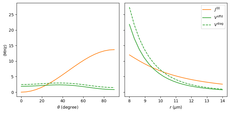
Finally, we can plot the results for the different distances and angles to reproduce the \(V^\mathrm{offd}\), \(V^\mathrm{diag}\), and \(J^{00}\) lines from the paper.

fig, axs = plt.subplots(1, 2, figsize=(8, 4), sharey=True)

axs[0].plot(theta_list, J00["theta"], "C1-", label=r"$J^{00}$")
axs[0].plot(theta_list, Voffd["theta"], "C2-", label=r"$V^\text{offd}$")
axs[0].plot(theta_list, Vdiag["theta"], "C2--", label=r"$V^\text{diag}$")
axs[0].set_xlabel(r"$\theta$ (degree)")

axs[1].plot(distance_list, J00["distance"], "C1-", label=r"$J^{00}$")
axs[1].plot(distance_list, Voffd["distance"], "C2-", label=r"$V^\text{offd}$")
axs[1].plot(distance_list, Vdiag["distance"], "C2--", label=r"$V^\text{diag}$")
axs[1].set_xlabel(r"$r$ ($\mu$m)")

axs[0].set_ylabel(r"(MHz)")
axs[1].legend()

fig.tight_layout()
plt.show()

\(M_\mathrm{tot} = +1\,\) subspace

To also reproduce e.g. the \(J^{+0}\) line from the paper, we can also consider the \(M_\mathrm{tot} = +1\,\) two-atom subspace, which contains the following states:

• |+, 0>

• |0, +>

And create the corresponding effective Hamiltonian for this subspace.

ket_tuples = [
    (ket_atoms["+"], ket_atoms["0"]),
    (ket_atoms["0"], ket_atoms["+"]),
]

eff_system = pi.EffectiveSystemPair(ket_tuples)
eff_system.set_perturbation_order(3)
eff_system.set_magnetic_field([0, 0, 60.7], "gauss")
eff_system.set_diamagnetism_enabled(True)
eff_system.set_minimum_number_of_ket_pairs(5_000)
eff_system.set_interaction_order(3)

eff_h_dict = {"theta": [], "distance": []}
for theta in theta_list:
    eff_system.set_distance(distance_default, theta, "micrometer")
    eff_h_dict["theta"].append(eff_system.get_effective_hamiltonian(unit="MHz"))

for distance in distance_list:
    eff_system.set_distance(distance, theta_default, "micrometer")
    eff_h_dict["distance"].append(eff_system.get_effective_hamiltonian(unit="MHz"))

Jp0 = {k: [eff_h[0, 1] for eff_h in eff_h_lists] for k, eff_h_lists in eff_h_dict.items()}

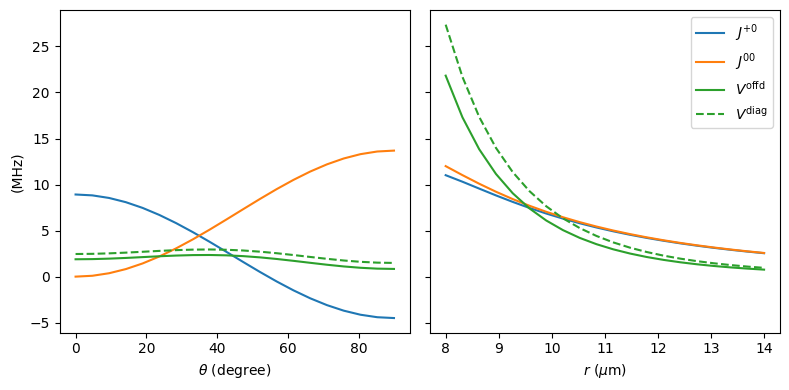
Plotting the results together with the previous results, we can reproduce the entire figure 2c) and d) from the paper.

fig, axs = plt.subplots(1, 2, figsize=(8, 4), sharey=True)

axs[0].plot(theta_list, Jp0["theta"], "C0-", label=r"$J^{+0}$")
axs[0].plot(theta_list, J00["theta"], "C1-", label=r"$J^{00}$")
axs[0].plot(theta_list, Voffd["theta"], "C2-", label=r"$V^\text{offd}$")
axs[0].plot(theta_list, Vdiag["theta"], "C2--", label=r"$V^\text{diag}$")
axs[0].set_xlabel(r"$\theta$ (degree)")

axs[1].plot(distance_list, Jp0["distance"], "C0-", label=r"$J^{+0}$")
axs[1].plot(distance_list, J00["distance"], "C1-", label=r"$J^{00}$")
axs[1].plot(distance_list, Voffd["distance"], "C2-", label=r"$V^\text{offd}$")
axs[1].plot(distance_list, Vdiag["distance"], "C2--", label=r"$V^\text{diag}$")
axs[1].set_xlabel(r"$r$ ($\mu$m)")

axs[0].set_ylabel(r"(MHz)")
axs[1].legend()

fig.tight_layout()
plt.show()