This page was generated from the Jupyter notebook c6_near_surfaces.ipynb. Open in Google Colab.

Dispersion Coefficients Near Surfaces

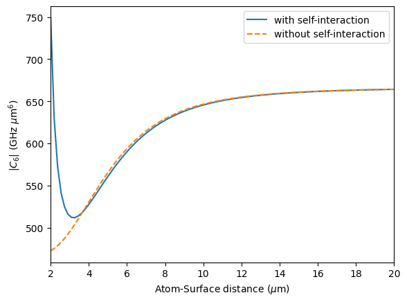
This jupyter notebook demonstrates how to compute the C6 coefficient near a surface using the pairinteraction library. It is comparable to the examples provided in the old pairinteraction software, which can be found here and reproduces the results from Phys. Rev. A 96, 062509 (2017). However, in this example here, we focus on the quantization axis point along the z-axis, which is perpendicular to the surface and interatomic axis.

# %pip install -q pairinteraction # Uncomment for installation on Colab

import matplotlib.pyplot as plt
import numpy as np
import pairinteraction as pi
from pairinteraction.green_tensor import GreenTensorSurface

if pi.Database.get_global_database() is None:
    pi.Database.initialize_global_database(download_missing=True)

ket1 = pi.KetAtom("Rb", n=69, l=0, j=0.5, m=0.5)
ket2 = pi.KetAtom("Rb", n=72, l=0, j=0.5, m=0.5)

distance_atoms = 10.0  # micrometer
distance_surface_list = np.linspace(0.05 * distance_atoms, 2 * distance_atoms, 100)

c6_list = []
for z in distance_surface_list:
    eff_system = pi.EffectiveSystemPair([(ket1, ket2), (ket2, ket1)])
    eff_system.set_magnetic_field([0, 0, 1], unit="gauss")

    gt = GreenTensorSurface(
        [0, 0, 0], [distance_atoms, 0, 0], z=-z, unit="micrometer", static_limit=True
    )
    eff_system.system_pair.set_green_tensor(gt)

    eff_h = eff_system.get_effective_hamiltonian(return_order=2, unit="GHz")
    c6 = -eff_h[0, 0] * (distance_atoms**6)  # GHz um^6
    c6_list.append(c6)

fig, ax = plt.subplots()
ax.plot(distance_surface_list / distance_atoms, np.abs(c6_list))
ax.set_xlabel("distance to surface / interatomic distance")
ax.set_ylabel("$|C_6|$ coefficient (GHz μm$^6$)")
plt.show()