Open as Jupyter notebook in Google Colab. In Google Colab, run pip install pairinteraction before the first notebook cell to install PairInteraction.

\(C_3\) and \(C_6\) Coefficients

The PairInteraction Python API comes with high-level functionality to calculate \(C_3\) coefficients (dipole-dipole) and \(C_6\) coefficients (van der Waals) without having to write much code. All functionality for calculating the coefficients are provided by the pi.C3 and pi.C6 classes:

• The constructor of the classes take the state of interest.

• The get method returns the coefficient.

• The classes determine automatically which states should be taken into account to obtain an accurate coefficient. To provide guidance what energy window or how many states in the pair basis should be considered, you can also use the method create_basis_pair(delta_energy, delta_energy_unit, number_of_kets) with either delta_energy or number_of_kets.

• If the coefficient should be calculated in the presence of e.g. a magnetic field, the set_magnetic_field method can be called before getting the coefficient. In general, the classes support similar setters as the pi.SystemAtom and pi.SystemPair classes.

If you are interested in calculating effective Hamiltonians beyond just the \(C_3\) and \(C_6\) coefficients, also check out the tutorial Effective Hamiltonians.

import matplotlib.pyplot as plt
import numpy as np
import pairinteraction as pi

if pi.Database.get_global_database() is None:
    pi.Database.initialize_global_database(download_missing=True)

Quickly get a \(C_3\) and \(C_6\) coefficient

In the following, we have a minimal example for calculating a \(C_3\) and \(C_6\) coefficient.

ket1 = pi.KetAtom("Rb", n=61, l=0, j=0.5, m=0.5)
ket2 = pi.KetAtom("Rb", n=62, l=1, j=1.5, m=0.5)

c3 = pi.C3(ket1, ket2).get("MHz um^3")
print(f"C3 coefficient between {ket1} and {ket2}: {c3:.3f} MHz um^3")

c6 = pi.C6(ket1, ket1).get("MHz um^6")
print(f"C6 coefficient of {ket1, ket1}: {c6:.3f} MHz um^6")

C3 coefficient between |Rb:61,S_1/2,1/2⟩ and |Rb:62,P_3/2,1/2⟩: -99.956 MHz um^3
C6 coefficient of (KetAtom(Rb:61,S_1/2,1/2), KetAtom(Rb:61,S_1/2,1/2)): -169208.708 MHz um^6

Angular dependence of the \(C_3\) and \(C_6\) coefficient

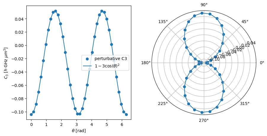
As a more sophisticated example, we calculate the angular dependence of the coefficients in the presence of a magnetic field along the quantization axis. For the angular dependence of the \(C_3\) coefficient, we recover the dipole pattern \(1-3\cos (\theta)^2\).

# Calculate C3 coefficients for different angles
thetas = np.linspace(0, 2 * np.pi, 40)
c3_coeffs: list[float] = []
for theta in thetas:
    c3_obj = pi.C3(ket1, ket2)
    c3_obj.set_diamagnetism_enabled(False)
    c3_obj.set_magnetic_field([0, 0, 20], "gauss")
    c3_obj.set_angle(theta, unit="radian")
    c3_coeffs.append(c3_obj.get("GHz um^3"))

# Plot the results
fig, axs = plt.subplots(1, 2, figsize=(10, 5))

axs[1].remove()
axs[1] = fig.add_subplot(1, 2, 2, projection="polar")

for ax in axs:
    ax.scatter(thetas, c3_coeffs, label="perturbative C3")
    ax.plot(
        thetas,
        -0.5 * c3_coeffs[0] * (1 - 3 * np.cos(thetas) ** 2),
        label=r"$1-3\cos(\theta)^2$",
    )

axs[0].legend()
axs[0].set_xlabel(r"$\theta$ [rad]")
axs[0].set_ylabel(r"$C_3$ [$h$ GHz $\mu m^3$]")

plt.show()

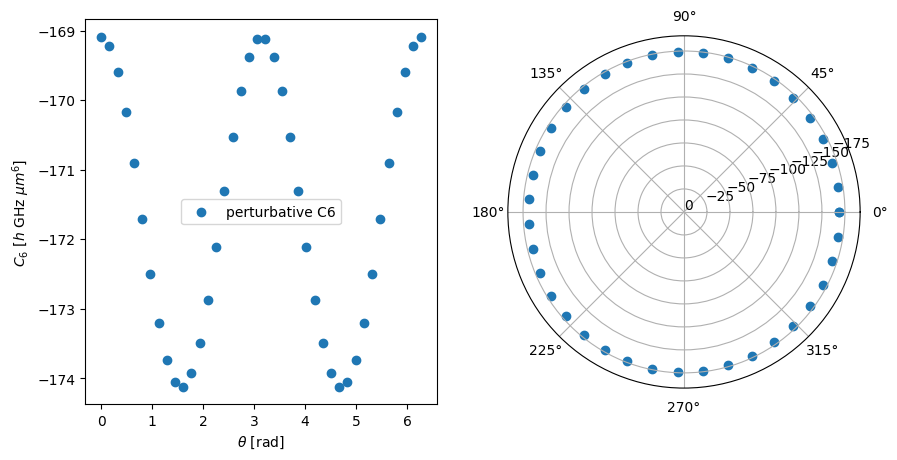
# Calculate C6 coefficients for different angles
c6_coeffs: list[float] = []
for theta in thetas:
    c6_obj = pi.C6(ket1, ket1)
    c6_obj.set_diamagnetism_enabled(False)
    c6_obj.set_magnetic_field([0, 0, 20], "gauss")
    c6_obj.set_angle(theta, unit="radian")
    c6_coeffs.append(c6_obj.get("GHz um^6"))

# Plot the results
fig, axs = plt.subplots(1, 2, figsize=(10, 5))

axs[1].remove()
axs[1] = fig.add_subplot(1, 2, 2, projection="polar")
# set the radial limits to 0 to the maximum negative value of c6_coeffs and add ticks
axs[1].set_ylim(0, min(c6_coeffs) * 1.1)
axs[1].set_yticks(np.arange(0, min(c6_coeffs) * 1.1, -25))

for ax in axs:
    ax.scatter(thetas, c6_coeffs, label="perturbative C6")

axs[0].legend()
axs[0].set_xlabel(r"$\theta$ [rad]")
axs[0].set_ylabel(r"$C_6$ [$h$ GHz $\mu m^6$]")

plt.show()