Open as Jupyter notebook in Google Colab. In Google Colab, run pip install pairinteraction before the first notebook cell to install PairInteraction.

Self-interaction of an atom near a surface

This notebook calculates the surface-induced self-interaction of a single rubidium Rydberg atom near a perfectly conducting plane. The self-interaction shifts the atomic energy levels and can also mix nearby Rydberg states when the atom is close to the surface.

import matplotlib.pyplot as plt
import numpy as np
import pairinteraction as pi
from pairinteraction.visualization.colormaps import alphamagma

if pi.Database.get_global_database() is None:
    pi.Database.initialize_global_database(download_missing=True)

The reference state is \(69P_{1/2}, m=1/2\) of rubidium. A single-atom basis is built around this state, and then the atom-surface distance is swept from \(1\,\mu\mathrm{m}\) to \(8\,\mu\mathrm{m}\). For each distance, a GreenTensorSurface object represents a plane below the atom with its normal along the \(z\) axis. The vacuum contribution has to be omitted, since the resulting free space contribution (Lamb shift) is already included in the atomic energy levels.

ket = pi.KetAtom("Rb", n=69, l=1, j=0.5, m=0.5)
basis = pi.BasisAtom.from_kets(ket, delta_nu=3, delta_l=3)

atom_surface_distances = np.linspace(1, 8, 300)

system_list: list[pi.SystemAtom] = []
for z in atom_surface_distances:
    system = pi.SystemAtom(basis)
    gt = pi.green_tensor.GreenTensorSurface(
        [0, 0, 0],
        [0, 0, 0],
        point_on_plane=[0, 0, -z],
        surface_normal=[0, 0, 1],
        unit="micrometer",
        without_vacuum_contribution=True,
    )
    system.set_green_tensor(gt)
    system_list.append(system)

pi.diagonalize(system_list)

energies_list = [
    system.get_eigenenergies(unit="MHz") - ket.get_energy("MHz") for system in system_list
]
overlaps_list = [system.get_eigenbasis().get_overlaps(ket) for system in system_list]

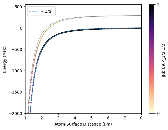
The plot shows the shifted eigenenergies as gray lines and colors each eigenstate by its overlap with the original \(69P_{1/2}, m=1/2\) state. At large distances, the branch connected to the reference state follows the expected static Casimir-Polder scaling proportional to \(1/d^3\), shown by the dashed fit. At short distances, the colored overlap reveals surface-induced mixing with nearby states.

fig, ax = plt.subplots()

ax.plot(atom_surface_distances, energies_list, c="0.5", lw=0.5)

x_repeated = np.hstack(
    [
        val * np.ones_like(es)
        for val, es in zip(atom_surface_distances, energies_list, strict=True)
    ]
)
energies_flattened = np.hstack(energies_list)
overlaps_flattened = np.hstack(overlaps_list)
sorter = np.argsort(overlaps_flattened)
scat = ax.scatter(
    x_repeated[sorter],
    energies_flattened[sorter],
    c=overlaps_flattened[sorter],
    s=5,
    cmap=alphamagma,
    zorder=-20,
)
cbar = fig.colorbar(scat, ax=ax, label=str(ket))
cbar.set_ticks([0, 1])

_id = system_list[-1].get_eigenbasis().get_corresponding_state_index(ket)
energies = np.array(energies_list)[:, _id]
a, b = np.polyfit(1 / atom_surface_distances**3, energies, deg=1)
energies_fitted = a / atom_surface_distances**3 + b
ax.plot(
    atom_surface_distances,
    energies_fitted,
    "C0--",
    label=r"$\propto 1/d^3$",
)

ax.legend()
ax.set_xlabel(r"Atom-Surface Distance ($\mu$m)")
ax.set_ylabel(r"Energy (MHz)")

ax.set_ylim(-2000, 550)
ax.set_xlim(1, 8)


plt.show()