Open as Jupyter notebook in Google Colab. In Google Colab, run pip install pairinteraction before the first notebook cell to install PairInteraction.

Stark map of Yb174

This notebook computes a Stark map for Yb174. The calculation follows the field-dependent energies near the \(49.7\,S_0\) Rydberg state and highlights how nearby states mix with this state in an applied electric field.

import matplotlib.pyplot as plt
import numpy as np
import pairinteraction.real as pi
from pairinteraction.visualization.colormaps import alphamagma

if pi.Database.get_global_database() is None:
    pi.Database.initialize_global_database(download_missing=True)

The reference state is the \(\nu = 49.7, S_0, m=0\) state. We build an atomic basis around this state, sweep a static electric field along the quantization axis, diagonalize the Hamiltonian for each field value, and store both the eigenenergies and the overlap of each eigenstate with the reference state.

ket = pi.KetAtom("Yb174_mqdt", nu=49.7, s=0, j=0, m=0)
basis = pi.BasisAtom(ket.species, nu=(ket.nu - 5, ket.nu + 5), j=(0, 7))

efields = np.linspace(0, 1.5, 200)
systems = [
    pi.SystemAtom(basis).set_electric_field([0, 0, efield], unit="V/cm") for efield in efields
]
pi.diagonalize(systems)

energies = np.array(
    [system.get_eigenenergies(unit="MHz") - ket.get_energy("MHz") for system in systems]
)
overlaps = np.array([system.get_eigenbasis().get_overlaps(ket) for system in systems])

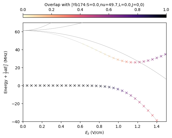
For the plot, the low-field quadratic Stark shift is removed by extracting an effective static polarizability from the energy at zero field and near \(0.5\,\mathrm{V/cm}\). The gray lines show the shifted eigenenergies, while the colored markers encode the calculated overlap with the reference \(S_0\) state. One can clearly see the avoided crossing with the nearby \(F_3\) Rydberg state, which mixes with the \(S_0\) state and causes a significant deviation from the quadratic Stark shift.

fig = plt.figure()
grid = fig.add_gridspec(nrows=2, ncols=1, height_ratios=[0.06, 2], hspace=0.10)
ax = fig.add_subplot(grid[1, 0])

ind0, ind1 = 0, np.argmin(np.abs(efields - 0.5))
energy0, energy1 = [
    systems[ind].get_corresponding_energy(ket, unit="MHz") for ind in [ind0, ind1]
]
polarizability = -2 * (energy1 - energy0) / (efields[ind1] ** 2 - efields[ind0] ** 2)
print(f"Polarizability: {polarizability:.2f} MHz/(V/cm)^2")

energies_shifted = energies + 0.5 * polarizability * efields[:, None] ** 2
ax.plot(efields, energies_shifted, c="0.5", ls="-", lw=0.25, zorder=10)

step_size = 6
x_repeated = np.hstack(
    [
        val * np.ones_like(es)
        for val, es in zip(efields[::step_size], energies_shifted[::step_size], strict=True)
    ]
)
energies_shifted_flattened = np.hstack(energies_shifted[::step_size])
overlaps_flattened = np.hstack(overlaps[::step_size])
sorter = np.argsort(overlaps_flattened)

scat = ax.scatter(
    x_repeated[sorter],
    energies_shifted_flattened[sorter],
    c=overlaps_flattened[sorter],
    s=30,
    cmap=alphamagma,
    marker="x",
    linewidths=0.8,
)

cax = fig.add_subplot(grid[0, 0])
fig.colorbar(scat, cax=cax, label=rf"Overlap with {ket}", location="top")

ax.set_xlim(0, 1.5)
ax.set_ylim(-40, 70)

ax.set_xlabel(r"$E_z$ (V/cm)")
ax.set_ylabel(r"Energy + $\frac{1}{2} \alpha E_z^2$ (MHz)")

plt.show()

Polarizability: 513.89 MHz/(V/cm)^2